Excel Online lets you view, edit and share your Excel workbooks from anywhere and it is free as part of Office Online or available for collaborating securely across your organization as part of an Office 365 subscription. We are pleased to announce several updates that help you with some of your most common spreadsheet tasks, including new ways to format data, use hyperlinks in your spreadsheet and explore data using PivotTables.
Read on for details about each one of these new and exciting improvements.
New ways to format data
Data comes in all shapes and forms. Excel Online now offers more number formats to display your data. To display the full list of format options, under the Home tab, click the Number Format drop-down and then select More number formats or right-click in a cell and select Format cells.
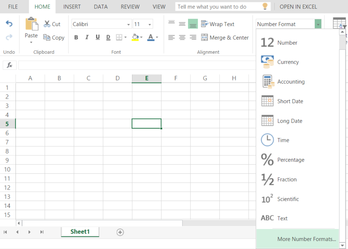
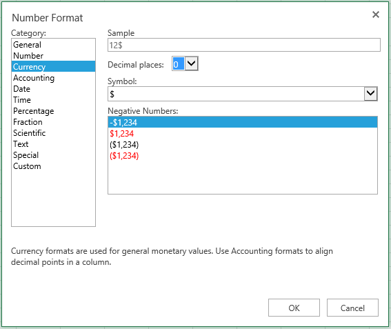
The beauty of using Excel Online is that it looks and feels like the Excel desktop experience you already know and love. Similarly, the Number Format dialog has the same options as the Excel desktop as we always try to keep the same and familiar user experience across all Excel platforms.
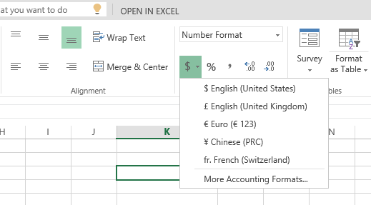
We know that currency formats are very common in spreadsheets, so we have made it easier for you to find the most common currency formats for your data. When you click the $ sign, under the Number Format section of the Home tab, you will find a list of the most common currencies with access to more accounting formats.
Connect your spreadsheet to more places using hyperlinks
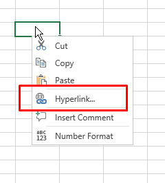
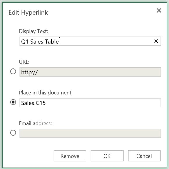
You can now do more with hyperlinks in your spreadsheet when you are using Excel Online. For example, in addition to connecting a URL, you can now hyperlink to a place in the document or an email address. To display the Edit Hyperlink dialog, click Hyperlink under the Insert tab. Alternatively, right-click in the cell and select Hyperlink.

Summarize and group data using PivotTables
PivotTables (and Pivot Charts) are one of the most productive tools that Excel has to offer because they make it quick and easy to summarize and group your tables of data in any way you like. With this update, you can do more with your PivotTables with settings to change the way you summarize your value fields. If you would like to see the average sales amount instead of total sales amount, then the Value Field Settings is your dialog. You can launch the dialog from the Value menu in the PivotTable setting pane.
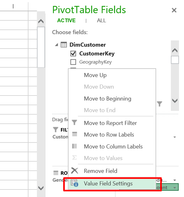
The Value Field Settings dialog consists of two tabs. The SUMMARIZE VALUE BY tab allows you to change the summarized value type.
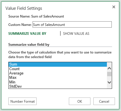

The SHOW VALUE AS tab enables you to change the type of calculation used in the PivotTable value fields. For example, instead of its absolute value, you can view the percentage out of the grand total.
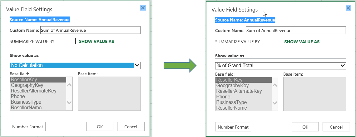

If you don’t like the value name, or if you wish to shorten it, you can rename it in the Custom Name text box.
Faster filtering in PivotTables with search
Just like regular tables in your workbook, you can filter data in your PivotTable for quick analysis. Now, Search dialog includes a Filter dialog to help you easily find the values you want to display. You no longer need to scroll through a list of hundreds or thousands of values to find what you are looking for. Search as you type makes your experience fast and friendly.

Saving your last viewed workbook
When you save a workbook and then open it with Excel Online later on, we keep you on the same sheet you last viewed, making it faster for you to keep moving with your work.
On-premises availability
On-premises users will also be able to benefit from the improved experience that we’re building for the cloud. All you need to do is have SharePoint deployed and then integrate it with the upcoming release of Office Online Server. In the future, you can expect to see frequent updates coming to on-premises in parallel to being released to the cloud.
Try them out yourself
Try out these new features and see how they can help you do more with Excel from anywhere!


