External Validity of Online Experiments: Can We Predict the Future?

November 20, 2024

Share this page

“It is difficult to make predictions, especially about the future”

– Yogi Berra (perhaps apocryphal)

How well can experiments be used to predict the future? At Microsoft’s Experimentation Platform (ExP), we pride ourselves on ensuring the trustworthiness of our experiments. We carefully check to make sure that all statistical tests are run correctly, and that the assumptions that underlie them are valid. But is this enough? All this goes to the internal validity of our experiments. What about their external validity [1]?

Suppose an experiment on Norwegian users shows that a change to your website increases revenue by 5%, with a tiny p-value and narrow confidence interval. How confident can you be that the treatment would increase revenue by 5% when shipped in Korea? Most data scientists would express reservations, urging that a separate experiment be run on Korean users. They would point out that Norwegian and Korean users likely have different preferences and user behaviors, and a change that users in one country love may be hated in another. In other words, they would question the external validity of the experiment and say that if you wanted to draw conclusions about the second population of users, you should run an experiment based on that population.

External Validity of the Future

However, at ExP we (along with every other online experimentation platform in the world) routinely assume the external validity of our results on a population that we never experimented on: users in the future. If we see a 5% revenue gain in an experiment one week, we assume that this means we will get revenue gains after we ship it, even though the future is different: user behavior may change over time, the type of users who use the product may change, other developers may ship features which interact with the first one, etc… How much should we worry about external validity here?

It’s a bit strong to say that we just “assume” this. We’re of course well aware both that the future is different, and that issues like “the winner curse” lead to systematically overestimating treatment effects [2,3]. We frequently validate our assumptions, by running reverse experiments (where the treatment reverts a feature) or holdout flights (where a holdout group of users are never shipped one or more new features) [4,5]. Our focus here is not on these sorts of checks, but rather on how often we should expect to have problems with external validity for users in the future.

External Validity and Surprises

Suppose we’ve collected data for a week and calculated a treatment effect and 3σ confidence interval for a metric. We’re planning to collect a second week of data and combine it with the first week of data to get an even better estimate. How confident are you that the new estimate will lie within that original 3σ confidence interval? How often would you expect to be surprised? Would you expect the surprises to come from external validity problems? Before reading on, try to form a rough estimate for your expectation.

Next Day External Validity: What Will Tomorrow Bring?

We started by looking at one-day metric movements. Most ExP experiments generate a 7-day scorecard which calculates treatment effects and their standard errors for all metrics relevant to the feature being experimented on. The scorecards typically also calculates those for each of the individual 7 days. We collected all 7-day scorecards generated by ExP over the course of a week. For every metric, for all 6 pairs of adjacent days, we compared the treatment effect estimates for those two days by calculating

\( z = \frac{\Delta_{t+1} – \Delta_t}{\sqrt{\sigma_t^2 + \sigma_{t+1}^2}}\)

Here Δ_t is the observed treatment effect on day t and σ_t is its standard error. This gave us several million treatment effect pairs, drawn from over a thousand online experiments.

Next-Day Deviations: a First Look

If the treatment effects from the two adjacent days are drawn independently from the same distribution, we should expect z to have the distribution of a unit width Gaussian. In practice, we might expect some positive correlation between the two, which would shift the distribution to smaller values of |z|. Comparing the distributions:

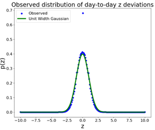
Daily deviations follow a Gaussian distribution for small z. — Figure 1: Day-to-day differences of treatment effects follow the expected normal distribution for |z|<3.

At first sight, it looks pretty good! There’s an extra spike in the observed distribution at z=0, which corresponds to a large number of metrics that have exactly 0 treatment effect on both days. Most of those come from poorly designed metrics that are almost always 0 in both control and treatment. But other than that, the fit looks quite close.

Next-Day deviations: a second look

Before we declare success and close up shop, let’s switch to a cumulative distribution function, and plot on a log scale:

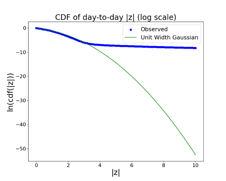
Distribution of differences between metric movements on adjacent days has deviations much larger than expected from the normal distribution well for |z| > 3, indicating external validity problems. — Figure 2: Day-to-day differences of treatment effects are much more common than normal distribution would predict for |z|>3.

Now we see that the match is pretty good for |z| < 3, but past that point, we start to get large |z| values much more than the Gaussian distribution would predict. As mentioned above, if there were positive correlations, we would have less values of large |z| than predicted by the unit Gaussian. But we have more. To show a few sample values from the graph above:

z	Observed CDF	Unit Gaussian CDF
1.96	3.4%	5.0%
3	0.25%	0.27%
4	0.09%	0.006%
5	0.07%	0.00006%
10	0.03%	2*10-²¹%

Table 1: Selected data points from the graph above, comparing observed CDF with the CDF of a unit Gaussian distribution.

Observing differences with |z| > 10 should essentially be impossible. In practice, it’s not common, but it does happen much more than it should: 3 out of 10,000 times isn’t a lot in absolute terms, but it’s a factor of 1.5*10¹⁹ too high!

Weekday and Weekend Effects

You might think that these large discrepancies come from comparing weekdays to weekends. For many business products, like Office or MS Teams, we would expect usage to be quite different on Friday and Saturday, for example. If we segment based on whether we’re comparing two weekdays, or two weekends, or a weekday to a weekend, we do find more large discrepancies when comparing a weekday to a weekend. But large discrepancies are found for all three categories:

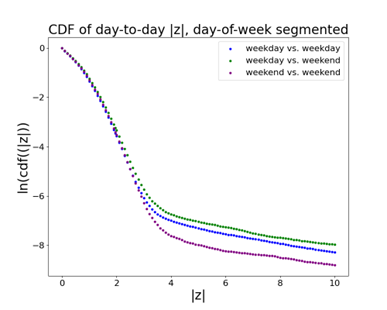
Deviations between different adjacent days are largest when comparing weekdays with weekends, but are qualitatively similar regardless of the day. — Figure 3: Day-to-day differences of treatment effects, segmented by whether we are comparing two weekdays, two weekends, or a weekday to a weekend.

This tells us that there’s a problem with using the data on day n to draw conclusions about day (n+1). It’s not a huge external validity problem. The assumption that today’s treatment effect is a reasonable predictor of tomorrow’s holds most of the time — but the bad predictions are worse than we’d naively expect. The distributions from which our samples are drawn on day n and day (n+1) are not the same, and that leads to large differences more often than you would expect. Another way of saying this is that if you looked at the standard error on day n, you would be overconfident about what you might see on day (n+1).

Differences between treatment effects on adjacent days follow the expected Gaussian distribution for |z|<3, but larger values of z occur much more often than expected.

This means that the true underlying treatment effects that we’re trying to measure are changing from day to day. These might be due to external factors, or they might be due to learning effects such as novelty and primacy effects [6]. We’ll return to this later – and show that systematic time trends such as from novelty and primacy aren’t the sole causes – but first let’s dig into the day-to-day movements.

Day-to-Day Volatility

This graph shows treatment effects on each of the first 7 days of an experiment at ExP (the metric and product have been anonymized):

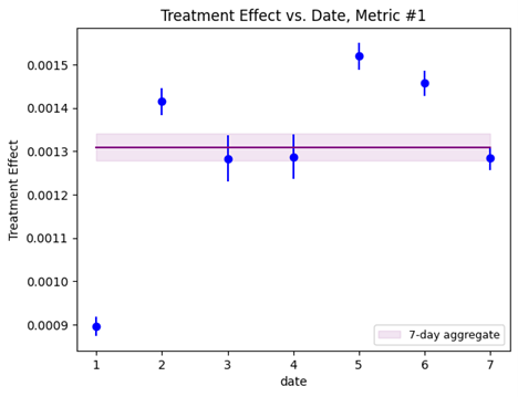
Time series of a metric that shows large shifts in treatment effects from day to day. — Figure 4: Time series for an anonymized metric, illustrating multiple shifts from day to day larger than expected by the daily error bars.

We see that there’s a lot of day-to-day volatility. The treatment effects shift up and down from day to day more than we would expect from the daily error bars. For example, on day #1 we are quite sure that the treatment effect is 0.0009, with a small error bar. But on day #5, we are sure that it’s 0.0015 – almost twice as much – again with a very small error bar.

The final result in the full 7-day scorecard is shown as a purple line, with the 95% confidence interval as a band around it. At ExP we warn customers that they should usually run their experiments for at least a week, to avoid weekday vs. weekend effects, or other events isolated to a single day. We next look to see if this gets rid of the external validity problem.

What Will Next Week Bring? (Not Necessarily Smaller Error Bars)

We next looked at all experiments at ExP over the course of a month that had 7-day and 14-day scorecards, to see what impact the addition of a second week of data had. We restricted ourselves to cases where the 7-day results were statistically significant (p < 0.05), since those are the metric movements our customers are most interested in. Since this is a biased sample, we also checked that the results were qualitatively similar when looking over all metric movements, without restriction by p-value.

The first big surprise, before even looking at the treatment effect values, is that when we go from 7-day to 14-day scorecards, the standard error decreases 83% of the time, and increases 17% of the time. Under the assumption that all data is drawn from the same fixed distribution, increasing the amount of data should almost always decrease the error bars. We’ve excluded from this analysis metrics that are cumulative, like “# of active user days,” restricting ourselves to metrics that don’t intrinsically grow with time, like “% of days a user is active.”

This is a clear sign that the data in the second week is drawn from a substantially different population than in the first week. We’re often not getting a more precise estimate of a point value. We’re instead mixing in samples from a new distribution and increasing the error bars.

Adding in a second week of data increases error bars on treatment effects 17% of the time.

This shows that even after getting a full week of data, we still don’t have a stable treatment effect. Whether that’s because the treatment effects are changing due to factors external to the experiment, or due to learning effects within the experiment is something we will address later, but the conclusion is still the same: we often do not have a stable measurement of the treatment effect even with a full week of data.

How Confident Can We be in Confidence Intervals?

Next, we looked at how often the 14-day result fell outside the 7-day 95% and 3σ confidence intervals. We call these “14-day surprises.” If we could get the true treatment effect, instead of just a 14-day result, this should only happen 5% and 0.3% of the time, respectively. The 14-day result instead fell outside 9% and 4% of the time. As a concrete example, for the time series we saw earlier in Figure 4, the 14-day result falls outside the 95% confidence interval, showing that even analyzing a full week of data didn’t fully capture the volatility of this metric.

You might object that the 14-day result isn’t the true treatment effect (and the very concept of the “true” treatment effect is rather nebulous, given that we’ve established that the distribution is changing over time). In reality, the 14-day result is a separate measurement, correlated with the 7-day result, since it’s based on a superset of the 7-day data. It’s not possible to generally calculate the probability of falling outside the 7-day confidence interval, because this correlation can be very complicated. For example, metrics can be user-level, with user activity spanning both weeks, or percentile metrics, which depend holistically on all the data.

How Often Should We be Surprised?

However, if the metrics are average metrics, with N samples in the first week, and N samples in the second week, then in the limit of large N, the probability of falling outside the 7-day confidence interval associated with z_α is 2*Φ(√2* z_α) where Φ is the unit Gaussian cumulative distribution function. This gives a probability of 0.56% for falling outside the 95% confidence interval, and 0.002% for the 3σ confidence interval. The probabilities are even smaller than when we earlier thought of the 14-day result as the true treatment effect, because the 14-day result has errors directionally correlated with those of the 7-day result, a result which should generally hold true even for more complicated metrics.

In the end, our concern here is less the precise theoretical value, and more that a typical data analyst takes a confidence interval as a good sign that “the right answer is probably in here,” and expects collecting more data to get them closer to “the right answer.” How likely are they to be surprised when they get more data? A 4% surprise rate for 3σ confidence intervals means a lot of surprises: we can’t be as confident in our confidence intervals as we would have initially expected.

When we add a second week of data, the new point estimate falls outside the 1-week 3σ confidence interval 4% of the time.

External Validity and Novelty: Why do Things Change Over Time?

We’ve established that the measured treatment effect changes over time, so that even a 7-day scorecard often doesn’t produce a stable measurement of the treatment effect. Does this occur due to factors external to the experiment, or due to learning effects?

Learning Effects

Alert readers may have been wondering if these changes can be attributed to learning effects, such as “novelty” or “primacy” [6]. We’re talking about the distribution changing with time, and it’s a well-known problem that users may take some time to adjust to online changes. Perhaps when a feature is introduced, users engage with it out of curiosity, making the feature look quite popular, but once the novelty has worn off, the gains fade away. Or perhaps the initial reaction appears bad, because users have difficulty adjusting to change, but once they get used to the new feature, the apparent regressions disappear or even reverse.

Given the following 7-day time series, most informed experimenters would warn that the treatment effect is systematically increasing with time, and that the 7-day confidence interval should be viewed with suspicion. They would say there’s a good chance that the 14-day result will lie above the 7-day confidence interval. (And in this case, they would be right.)

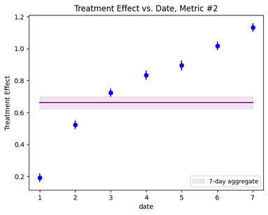
Time series of a metric that shows a systematic time trend, with treatment effects increasing every day. — Figure 5: Time series of treatment effects showing a systematic time trend.

Is this the cause of the 14-day surprises that we saw earlier? When we visually scan through the time series for the 14-day surprises, we do see many graphs with systematic time trends, such as in figure 5, but we also see many graphs like that in figure 4, where the results move up and down randomly from day to day.

Kendall’s Tau Statistics

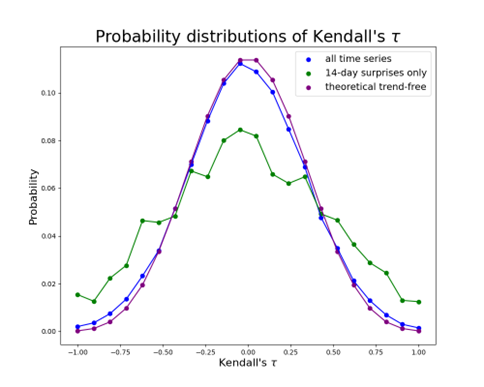
Learning effects should generally result in systematic trends, with treatment effects monotonically increasing or decreasing with time. To quantify our observation that the 14-day surprises are from a mixture of causes, we plot the distribution of Kendall’s τ statistic on the 7-day series [7]. This statistic is a measure of how “time-trendy” the data is: it’s +1 if the data is monotonically increasing, -1 if it’s monotonically decreasing, and otherwise takes on some intermediate value depending on how consistently the data is trending up or down.

Figure 5 shows the distribution of Kendall’s τ across all 7-day series in blue. The theoretical distribution of Kendall’s τ that we should expect if there were no time trends, so that all 7! permutations of time series are equally likely, is plotted in purple. (For simplicity we’re removed a small number of time series with ties between treatment effects on different dates.) When looking over all time series, larger absolute values of τ are slightly preferred, showing that some time trends exist, but that the overall bias is relatively small.

Distribution of Kendall's Tau statistics. When looking at all metric time series, the distribution is close to the theoretical trend-free distribution, with only a slight bias towards time trends. The 14-day surprises have a much more substantial deviation, but also still have a fair amount of weight for low, trend-free Kendall's tau values. This indicates a mixture of external validity issues and learning effects. — Figure 6: Distributions of Kendall’s τ . The distribution over all time series looks similar to that from the theoretical trend-free distribution. The 14-day surprises have a shift towards larger values of | τ |, but still a significant number of low values of | τ |, showing that a large number of surprises cannot be attributed to learning effects

Learning Effects vs. External Validity

When we restrict to the cases where we have 14-day surprises (14-day results outside the 7-day 95% CI) the distribution shifts significantly to larger absolute values of τ, showing that learning effects are responsible for a significant number of the surprises. However, there is still a healthy portion of the distribution at low values of | τ | that would occur naturally even with a trend-free distribution, confirming our observation that many of the time series look like those in figure 4, with no observable time trend, and thus no sign of learning effects. Novelty and primacy effects are significant causes of treatment effects changing over time but are not the sole causes.

Conclusions

This shouldn’t be a cause of great pessimism or despair about the value of statistical tests or online experimentation. The external validity issues that we’ve seen here are the exception, not the norm. Extrapolating from statistical tests on past data to the future works most of the time, and online experimentation is still the best way to measure the impact of your changes and estimate what will happen when you ship them.

But it should be a cause for at least some healthy skepticism about the future impact of your changes. If you really want to be sure about that impact in the future, you need to continue to measure it, with extended experiment durations, reverse flights or holdout experiments. Observing much higher day-to-day volatility in the treatment effects than you would expect from the single day standard errors provides a reasonable starting point for detecting cases where you need to do this.

Bibliography

[1] “The Importance of External Validity,” A. Steckler and K. R. McLeroy, Am. J. Public Health, 98: 9-10 (2008)

[2] “Selection Bias in Online Experimentation,” M. Shen, Medium.com (opens in new tab)

[3] “Winner’s Curse: Bias Estimation for Total Effects of Features in Online Controlled Experiments,” M. Lee and M. Shen, KDD ’18: Proceedings of the 24th ACM SIGKDD International Conference on Knowledge Discovery & Data Mining, p.491-499

[4] “Holdout testing: The key to validating product changes,” statsig.com blog (opens in new tab)

[5] “Holdouts: Measuring Experiment Impact Accurately,” geteppo.com (opens in new tab)

[6] “Novelty and Primacy: A Long-Term Estimator for Online Experiments,” S. Sadeghi et. al., https://arxiv.org/abs/2102.12893 (opens in new tab)

[7] Kendall, M. (1938) A New Measure of Rank Correlation. Biometrika, 30, 81-89